Investigating Bitcoin Market Crashes With Option Probabilities

This research piece was conducted in conjunction with @epsilonsized and @tristan0x from Zeta Markets, a cutting-edge DeFi options platform built on Solana.

Whether it be scanning through an early stage token’s Discord server for alpha leaks or studying on-chain ETH data, the best crypto investors rely on some form of data analysis in their investment decision process. Given these two methods are already quite well known, we wanted to explore a novel signal extracted from the crypto options market and determine whether it contains any useful insights. The purpose of this research piece is to derive the theoretical implied probabilities from Deribit’s BTC option prices and analyze whether we can use this rarely used signal in the alpha generation process.

We’ll start with a high-level overview of risk neutral option probabilities, review several case studies of BTC market crashes, and lastly investigate whether the probabilities can be used for predictive modelling.

Part 1: Overview of Risk Neutral Probabilities

Any liquid option market will provide hidden clues baked into the price of these derivatives. In this analysis we’re interested in extracting the probabilities implied by the options market to get a sense of where BTC will be trading at maturity. Similar to how traders derive implied volatility from the price of an option, we can also use mathematical formulas to reverse engineer the implied probability distribution. For the more technically inclined, this process will involve solving for the probability density function by partially differentiating the Black-Scholes formula (the mathematical logic and approach is described in the Appendix).

We can think of the risk neutral probability as a key tool to compute the fair price of any derivative. Specifically it is the set of probabilities at which the price of the derivative is equal to the discounted expected value of its future payoffs. Let’s consider the following trading opportunity below:

• Win $100 when the Lakers win the ‘22 championship. We think there is a 30% chance this will happen
• Lose $20 in all other cases
• The Expected Value at Expiry = ($100 x 0.30)  + (-$20 x (1 - 0.3)) = $16.00
• Using a 0% interest rate for simplicity, this security should be valued right now at $16.00

Now what if we knew the price the security was trading at, but not the risk-neutral probabilities? We could actually reverse engineer the equation, and get to the risk-neutral probabilities by using the price of the security. If the security was trading at $40, that tells us the world expects ($100 x p) + (-$20 x (1 - p)) = $40.00.

In this case, the risk neutral probabilities for each outcome solve to 50% and 50%, as we can tell what probabilities the rest of the world are using to price this security (go Lakers!). Using this example as a framework, we can utilize the probabilities derived from the option prices to gain insights on how traders are thinking about the market. When prices are in a bullish up-trend, option prices should reflect a higher probability in the upper strikes. Conversely, when prices are bearish, the options market will adjust accordingly and suggest higher probabilities for lower prices.

It is worth mentioning that the risk-neutral probability can, at times, deviate significantly from real-world probabilities due to investor risk preferences. The risk-neutral probabilities calculated by this measure may be quite different, as we will highlight in examples such as March 2020.

Part 2: Case Studies

A) March 2020: Black Thursday

Given this was one of the most extreme moves in BTC’s recent history, we'll explore how the probabilities reacted during this time. In this case we’re analyzing how the probabilities evolve up to expiry for a maturity with roughly 30 days.

Before the crash around February 25, 2020, BTC was slowly declining given the market-sell off pressure from COVID worries. Near the end of the option’s maturity on March 26, 2020, BTC’s price had already crashed hard, however, partly recovered from the Black Thursday daily low of $4.7k. As the expiry approached maturity, the probability distribution became much narrower — this makes sense because as we get closer to expiry, the market is pricing in much tighter price moves near the current spot price. In other words, the green curve had more width to it because it had much more time for the prices to move, whereas the red curve narrowed sharply due to the limited time remaining.

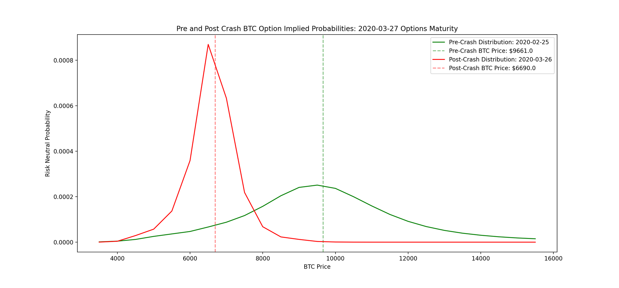
In either case it’s evident the peak probability distribution value will be near the current spot price of BTC. This makes sense because it suggests the market’s best estimate for the future price of BTC is the current price itself.

We can also take a look at the 3D plot to showcase how the probability distribution changes over time. Notice how the probability distribution shifts aggressively during the Black Thursday event with probabilities spiking up very fast but then to mean-revert just as quick. This aligns with the market behaviour of mean-reversion — ie: when an asset experiences a sharp jump in either direction, it’s likely the market will mean-revert which is evidenced by this 3D plot.

Also observe a graph of the density with respect to moneyness (what we’ve computed here as Strike/Spot). The risk-neutral density is dominated by where spot is at the current time, but when we normalize for the current spot price we’re able to observe what investors think are the probabilities of spot going up or down. On March 13th although BTC already crashed to $4.7k, the implied probability of the spot price falling another 20% (signified by the 0.8 moneyness point) actually doubled. The market was saying that BTC was even more likely to go down again (and was very wrong)!

B) May 2021: Summer Correction

This was the worst drawdown during 2021 with BTC crashing from nearly $56k to $35k during May resulting in nearly a 40% peak to trough loss. Many attribute this selloff to Elon Musk reversing his opinion on BTC due to environmental concerns. Additionally, during this time there was a lot of bearish news coming out from China in regard to restrictions on crypto trading in the country.

In this case we’ll start our analysis on May 1, 2021 and use the May 28, 2021 option expiry to see how the risk neutral probability distribution changes over time. Similar to above, we’ll focus on an option maturity of around 30 days at the inception for this analysis. Before the crash, the probabilities peaked near $60k with a relatively flat distribution. This makes sense because with nearly 30 days to expiry, the market was less certain where prices would settle which explains the width in the probability curves.

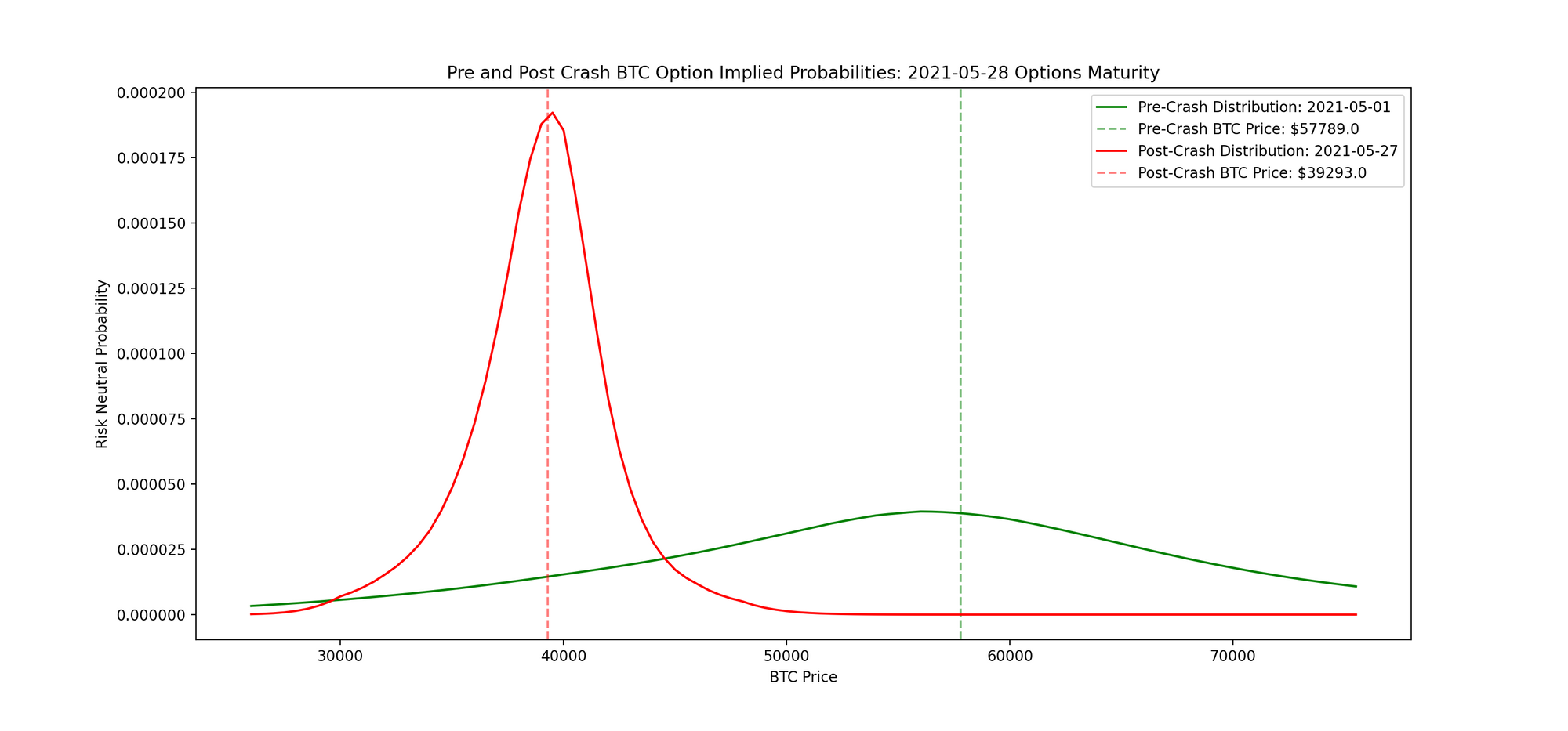
After the massive volatility events in May 2021, similar to the above analysis we can see the probability curve starts to narrow near the current price of BTC. This is a common behaviour to expect especially as the option maturity reaches expiry. In the moneyness dimension, it's evident this selloff was much less panicked than March 2020 as implied densities +/- 10% stayed steady, and participants did not greatly change their opinions on the price process of BTC.

C) September 2021 Correction

Recently we saw a violent crash in the price of BTC which resulted in nearly a 20% drawdown within the course of several hours. This price volatility was mostly attributable to over-leveraged crypto futures markets which resulted in a cascade of liquidations. The process of exchanges auto-liquidating traders with underwater equity balances is the primary reason why crypto prices are so volatile during these events as forced selling further magnifies any decline.

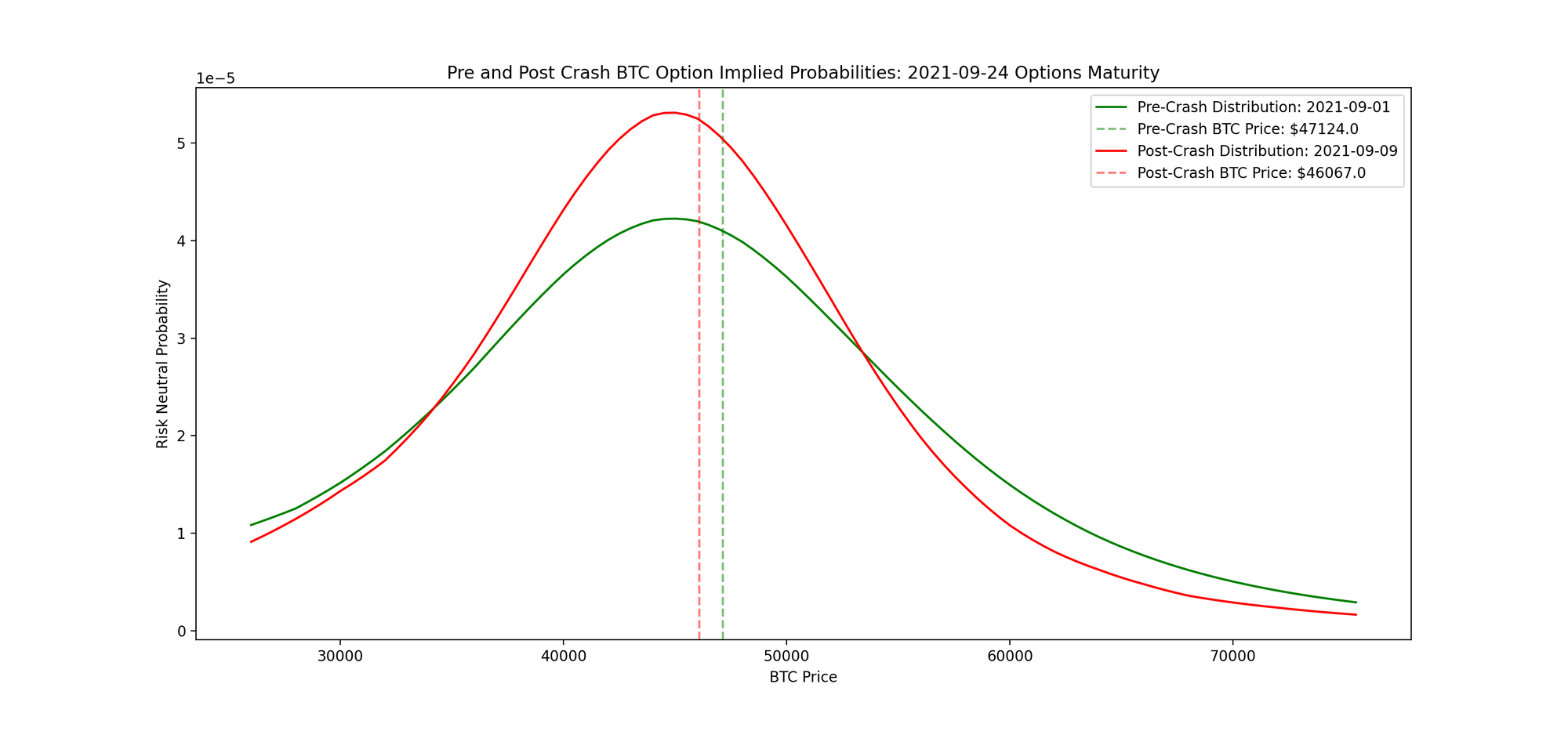
In this case we’ll begin our analysis on September 1st and reference the September 24, 2021 options expiry which gives us roughly 25 days to maturity. Given this maturity is still live, we can see in real-time what the probability curve currently looks like. Similar to before, the post-crash probability distribution has a narrower peak at a lower BTC price. Furthermore, near the upside tails we can see the pre-crash probabilities were slightly higher for OTM strikes (ie: 60K+). An interesting phenomena we noticed was the post-crash downside tails had lower probabilities than pre-crash. This is peculiar behaviour because if we’ve already crashed down then it’d be reasonable to expect the probabilities for lower strikes to correspondingly increase.

Part 3: Does This Generate Alpha?

Although this analysis may look interesting at the end of the day we need to find a way to make money from this signal. The best use-case for these risk-neutral probabilities would be to see if they have any predictive power in the future price change of BTC. For this analysis we will focus on the recent September “flash-crash” but instead use hourly data to compute the probabilities as this will give us more data points.

A simple check for detecting this feature’s predictive power would include running a regression against the price return series of BTC vs the change in risk-neutral probability near the ATM strike. As we observed above, in most cases the ATM strike had the highest probability, therefore as an approximation we can use the maximum probability at each hour.

Let’s review the steps for this analysis:

1. Create a time-series with the percentage change for ATM risk neutral probability and spot BTC on an hourly basis.

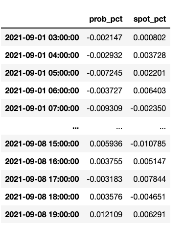
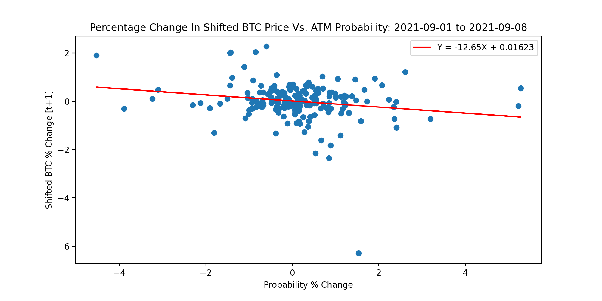
2. We will treat the probability percentage as our “x-variable” and use it to predict the future percentage change in BTC which is the “y-variable”. The BTC return values will be shifted back by one hour to ensure we’re predicting on future data to reduce the risk of lookahead bias.

3. Run a simple linear regression to see if there are any insightful patterns. From a visual glance there is a slight negative relationship between the two variables, however, this relationship is very weak. Although the risk neural probability coefficient in this regression is statistically significant at a 95% confidence level, this regression’s r-squared value of only 0.036 doesn’t successfully highlight the predictive attributes of this feature.

Based on this analysis it doesn’t appear the ATM option probability has any material predictive insight towards the future price changes of BTC. Further discussion below will showcase why this may be so and when we may begin using the risk neutral probability more reliably in future alpha modelling.

Key Takeaways

Currently the crypto options market is not large enough to materially move the underlying spot market (there is some degree of influence on the spot market near 8AM UTC at major expiries as indicated in this article). Therefore most signals we extract from crypto option data will likely not have any useful predictive insight until this market grows to materially influence spot markets on a consistent basis. As an example, futures in crypto have a considerable impact on spot markets especially during volatile times. For that reason, it currently makes more sense to use futures specific data (ie: funding rates, leverage ratios, open interest etc.) rather than options data when building a predictive model.

Another important thing to keep in mind is that the option probability distributions are also heavily influenced by non-fundamental factors such as the risk tolerance of market-makers and current options flow. It could well be the case that market participants have affected the implied density distribution such that it isn't reflective of real world distributions, which should mean there is a volatility arbitrage opportunity available.

Overall, as the crypto market gets more institutionalized with new sophisticated investors, market participants will need to become savvier with their approach on extracting edge. This will naturally result in alpha decay for existing signals but will force investors to become more creative with their process.

Appendix A: Modelling Steps

1. Calculate the risk neutral density using the formula as indicated in Appendix B. This is done by feeding in various option input parameters (ie: strike, underlying price, volatility, time to maturity, and interest rate).
   
2. At the start of each case study choose an option maturity to analyze across time. For example, in the case of the March 2020 Black Thursday analysis, we start the analysis on February 25, 2020 and end on March 27, 2020. As a result, we’re referring to a ~30 day maturity at inception which will gradually expire by March 27.
   
3. For each daily observation, we calculate the risk neutral probabilities across every strike in the selected maturity. Given the raw Deribit data only has discrete strikes, we’ll have to linearly interpolate the strikes and implied volatilities to allow for a smoother curve when calculating the implied probability distribution.
   
4. Repeating this same process for each day allows us to generate a 3D plot of the probability distributions across time.
   

Appendix B: Risk Neutral Distribution Formula

The following mathematical formula is referenced from Espen Haug’s book, “The Complete Guide To Options Pricing Formulas.” There are two interesting things to note about this formula:

• We can refer to the risk neutral density as “strike gamma” because we are taking the second derivative of the option price w.r.t strike. With regular spot gamma we are taking the second derivative of the option price w.r.t spot.
• Similar to spot gamma, the risk neutral density will be the same for both calls and puts (provided the strikes are the same)

Disclaimer: Nothing mentioned in this article constitutes as financial advice. LedgerPrime is an investor in Zeta Markets. Opinions expressed are solely my own and do not express the views or opinions of LedgerPrime.