How to Land a Plane (Using Math): A Quantitative Look at Real-World Glide Slopes
Introduction
During my early instrument-training flights, the turn from base to final—rolling wings level and aligning precisely with the runway always stood out as one of the most demanding moments. Alongside take‑off, this phase demanded the highest level of precision, focus, and composure.
For visual landings, my instructor always reminded me to keep the runway fixed in the windscreen so it neither rises nor sinks—an intuitive cue for a stable descent. Under instrument conditions, that visual reference is replaced by a technical standard: the 3‑degree glide path. Nearly every published IFR approach specifies this angle, giving pilots a consistent target for planning and executing safe, stabilized descents. In practice, the 3‑degree glide slope functions as a simple yet essential anchor during one of flight’s most critical phases.
Today, with extensive ADS‑B flight data available through public APIs, we can examine how closely real‑world approaches adhere to this benchmark. By reconstructing glide paths from live flight tracks, this project asks a straightforward but meaningful question: Does actual approach behaviour match the 3‑degree standard? The analysis aims to quantify that alignment and highlight any systematic deviations—offering an empirical view of how theory meets practice on final approach.
Part 1 | Instrument Approaches in Context
A pilot can depart the same runway but operate under two very different regulatory frameworks: Visual Flight Rules (VFR) or Instrument Flight Rules (IFR). Both demand strong stick‑and‑rudder skills, yet they place the pilot in distinct operational worlds. Under VFR, navigation is driven by what you see outside the cockpit; under IFR, you rely on the six basic flight instruments (the classic “six‑pack”) and a suite of electronic aids to stay upright and on course—often with little or no outside view.
Whenever you board an international airline flight, rest assured the crew is flying IFR. No one wants a wide‑body plane climbing through thick clouds while the pilots “feel it out.” Spatial disorientation is real and unforgiving; Kobe Bryant’s helicopter accident is a stark reminder. My own instructor once had me close my eyes and hold what felt like level flight. Thirty seconds later we were creeping into a steep, pre‑stall bank—proof enough that inner‑ear sensations can betray you!
For IFR approaches, the classic technology is still the Instrument Landing System (ILS). It broadcasts two independent radio beams:
- Localizer – lateral guidance to centerline.
- Glide slope – vertical guidance down a predefined descent path.
By aligning both needles (or bars), the aircraft remains on a stable “rail” all the way to decision altitude.

A 3‑degree glide path has become widely used because it balances obstacle clearance, passenger comfort, and braking distance. Consider the CYVR ILS RWY 13 plate: the published glide path is 3°. Even the step‑down altitudes between waypoints—IGVAS to DATSI, DATSI to PETKO—align with that same geometry, saving pilots from having to do mid‑air trigonometry. For instance, at 7 NM from the runway (DATSI), a pilot should be at or slightly above 2,340 ft MSL to glide down a ~3‑degree slope.

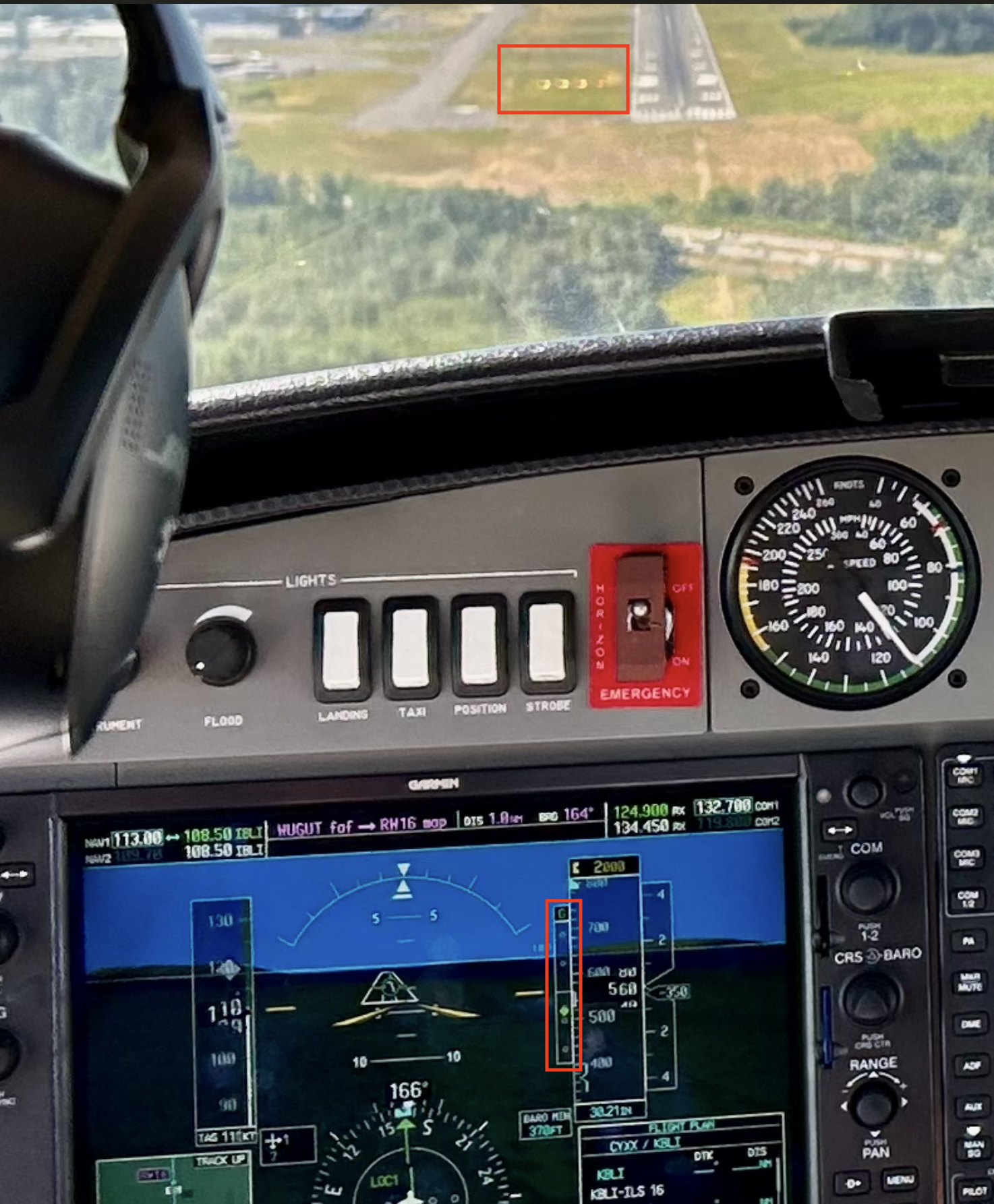
From a personal standpoint, mastering a hand‑flown ILS was a cornerstone of my instrument training. It underscored just how precise and stable a descent path must be. The image below captures me in a DA‑42 light twin, flying the ILS into Bellingham (KBLI) for RWY16. Astute aviators will spot that I am slightly high on the glide path—three white PAPI lights and a half‑dot deviation on the G1000 confirm it, as illustrated in the image below. On this clear, sunny day, the margin was forgiving—but in actual cloudy conditions, as illustrated below, focus would remain on the instruments, with only brief checks outside for the first glimpse of runway lights.
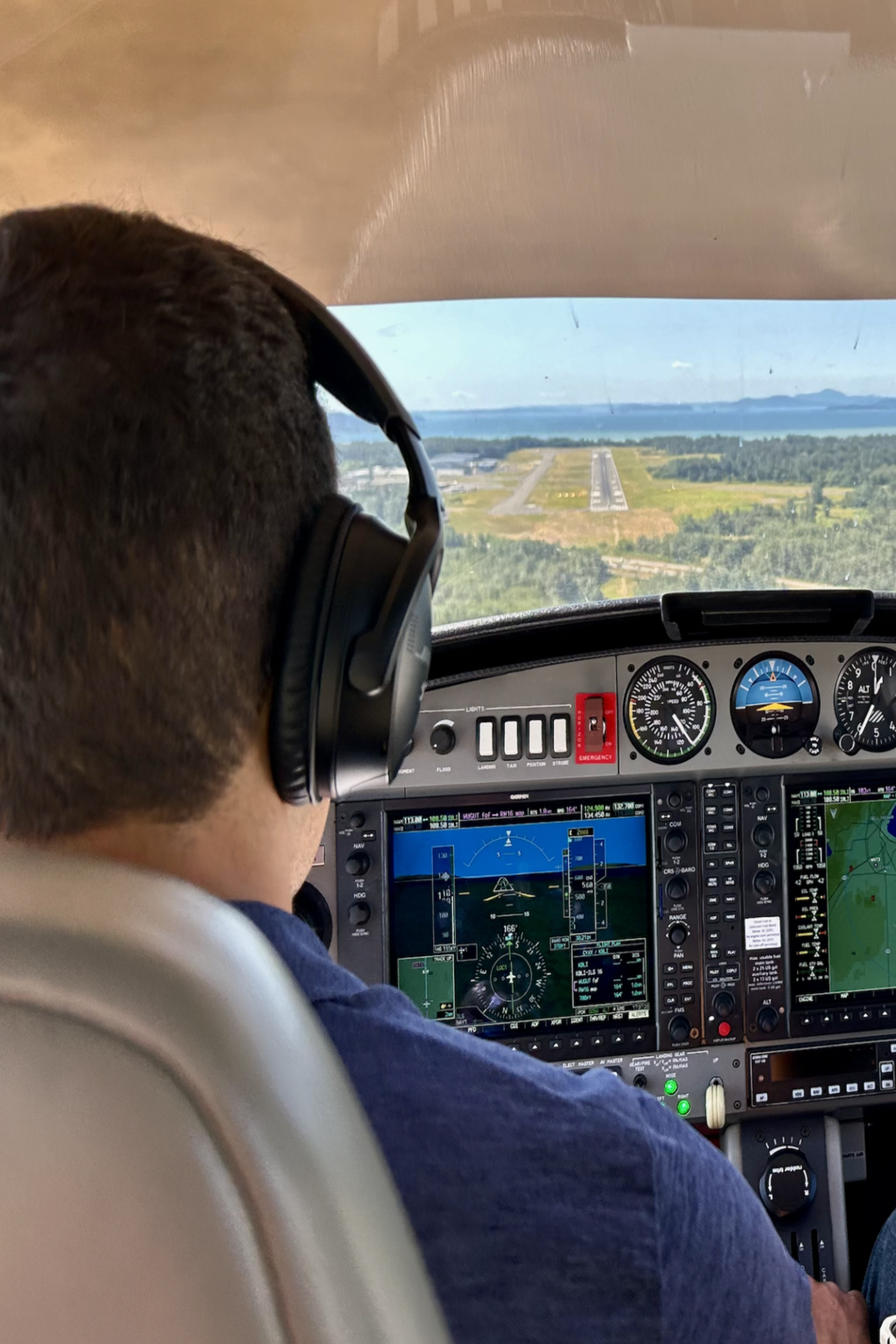
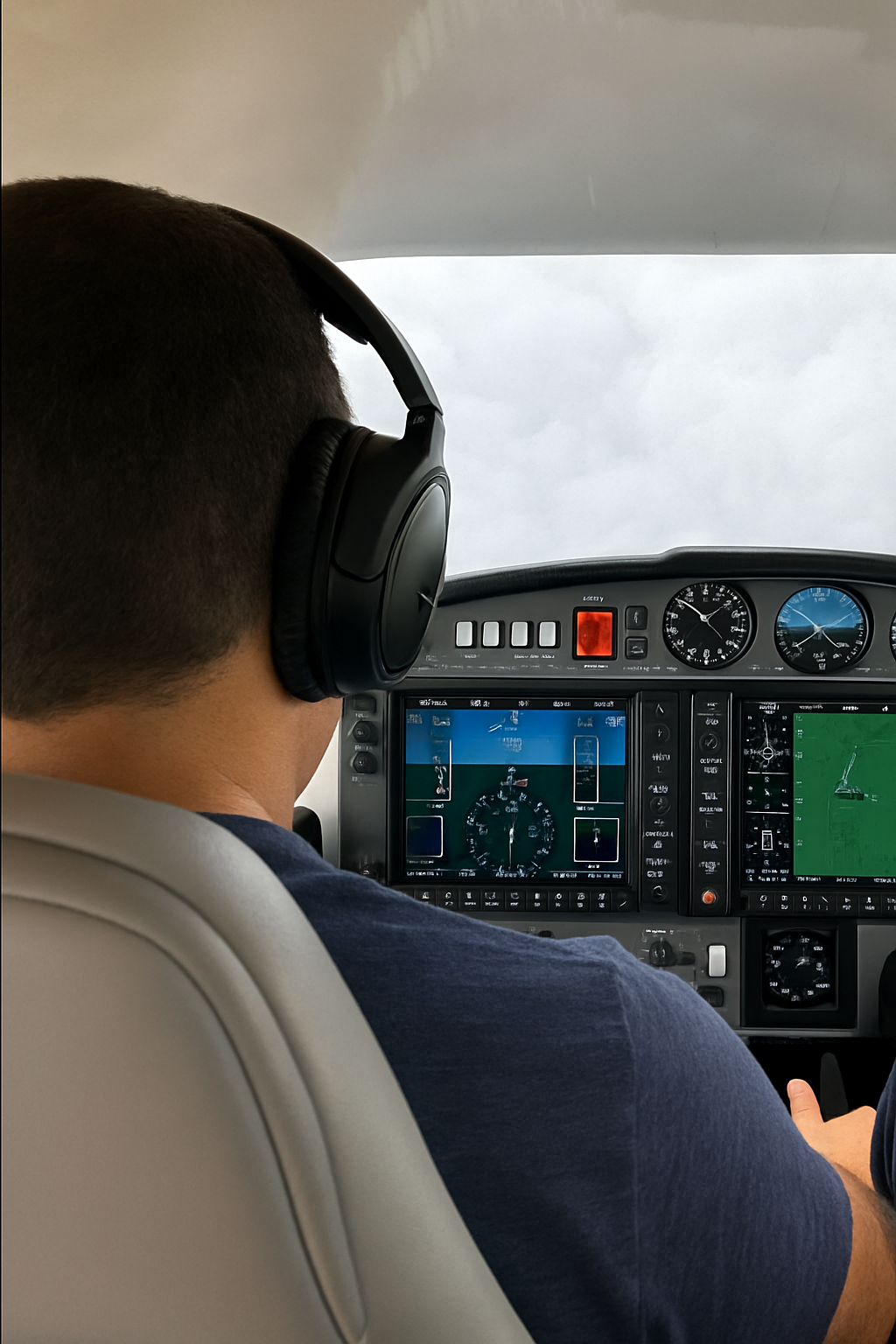
The AI-simulated image on the right illustrates how, in thick cloud, relying on instruments is crucial—there’s no time to navigate by visual means!
Thousands of planes execute IFR approaches every day. With global ADS‑B coverage and publicly available API data, we can now measure how closely these approaches adhere to the published 3‑degree standard. By reconstructing final‑segment flight profiles, we can score approach stability, quantify systematic deviations, and provide data‑driven insights for training and safety—testing whether real‑world operations match textbook theory.
Part 2 | Methodology and Modelling Approach
To assess approach quality, each flight’s vertical profile is benchmarked directly against the published IFR chart for its runway. For every track point on final, we compute two values:
- Published altitude derived from a 3‑degree reference line (or the step‑down altitudes on the plate) at that same distance from threshold.
- Actual altitude from the ADS‑B record.
The difference between the two yields an instantaneous glide‑slope error. Aggregating these errors across the approach lets us quantify how faithfully the aircraft followed the charted path and compute an empirical glide‑slope for every segment. Repeating this process flight‑by‑flight produces a clear, data‑driven score of approach stability and overall glide‑slope conformance.
- Data Sourcing
To keep the scope focused, I limited the dataset to flights arriving at Vancouver International Airport (CYVR) between January 1 and January 10, 2025. Over those ten days, roughly 3 000 individual flights were tracked. All trajectory points including timestamps, latitudes, longitudes, and recorded altitudes were pulled directly from the FlightRadar24 API. This provided the raw material for reconstructing each final segment and benchmarking it against the published ILS profile.
- Approach Plate Selection and Assumptions
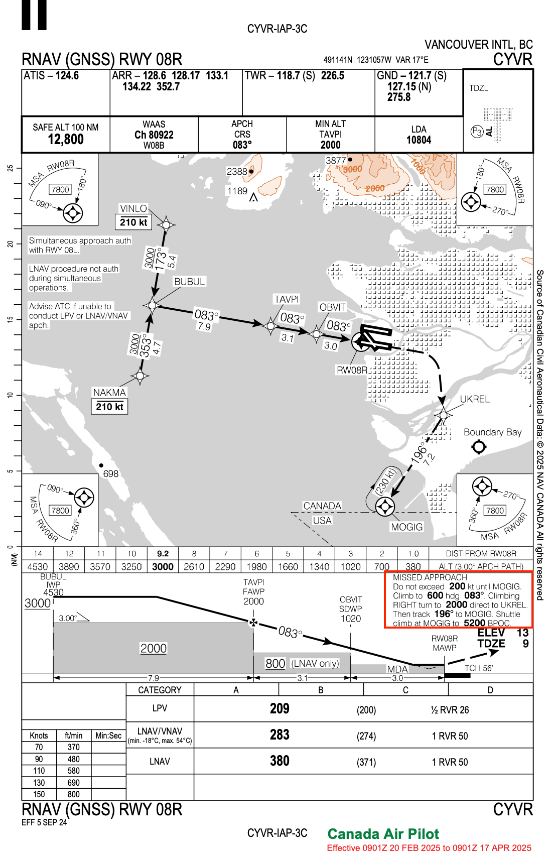
For this analysis, we selected the primary instrument approaches into CYVR—ILS on Runways 26L/26R and 08L/08R. We assume arriving flights adhere to those published ILS procedures. In practice, some aircraft may fly RNAV (GPS), visual, or vector‑guided approaches, but their vertical profiles converge closely in the final segment.
For instance, the RNAV approach for Runway 08R shares nearly the same 3° descent as ILS 08R, differing only by a few dozen feet at specific waypoints. Given our focus on vertical descent behaviour relative to the glide slope, this approximation has minimal impact. Operational variances—wind, ATC vectors, or pilot technique—introduce far greater altitude deviations than the minor plate discrepancies. This assumption therefore offers a practical balance between modelling rigour and real‑world complexity.
- Calculate Distance From Runway
For each flight, we use ADS‑B latitude, longitude, and altitude points to map the aircraft’s final segment. Although FlightRadar24 tags the runway in use, we still compute the precise distance from each position to the runway threshold. By determining this distance in nautical miles at every timestamp, we build a continuous profile of how the aircraft closes in on the runway.
We calculate those distances using the Haversine formula, which accounts for Earth’s curvature when measuring between two latitude‑longitude pairs. To improve resolution, we interpolate positions and altitudes to one‑second intervals, then apply the Haversine calculation iteratively. The result is a highly granular, second‑by‑second track of distance versus altitude for each approach.


Source: Wikipedia and Sketchplanations
It’s important to note that while the Haversine method is reasonably reliable over typical final-approach ranges (10–20 NM), it can introduce minor errors when the aircraft is very close to the runway threshold. For future research, more advanced methods—such as Python’s GeoPy library, which includes packages that model the Earth’s curvature more accurately could be used to improve precision.
- Calculating Instantaneous Glide Slope
With distance and true AGL altitude in hand, we can compute the instantaneous glide‑slope angle at each point using an arctangent of vertical over horizontal separation. While our horizontal distances come from a curvature‑aware Haversine calculation, this trigonometric step treats the ground as flat which is a reasonable simplification within the last 10 NM of final approach.

To ensure consistent comparisons across flights, we focus our analysis around a common reference point: approximately 6.1 nautical miles from the runway threshold. This distance corresponds to the Final Approach Fix (FAF) on all published ILS approaches into CYVR—a critical waypoint in the descent profile. At the FAF, aircraft are expected to be at or near a specified altitude, typically around 2,000 feet ASL, as outlined in the IFR approach plates. By calculating the instantaneous glide slope at this point for each flight, we can generate a distribution of real-world glide slopes and assess how closely they align with the theoretical 3-degree standard. In essence, this gives us a consistent benchmark to evaluate whether each flight is tracking the expected descent path at a key point in the approach.
Part 3 | Analysis of Model Output
1. Landing Score
To objectively assess each flight’s approach quality, we can develop a scoring system that quantifies how closely an aircraft followed the expected glide path. This required a few practical assumptions—most notably, that arriving aircraft generally adhere to the published instrument procedures for their assigned runway.
While this assumption isn’t perfect (as real-world ATC may issue vectors or clear aircraft for visual or RNAV approaches), it remains reasonable. The majority of approaches into CYVR—especially those guided by ILS—are designed around a nominal 3-degree glide slope. Even alternate procedures, such as RNAV (GPS) approaches, closely mirror this angle in the final segment. Given the emphasis on stabilized approaches in modern airline operations, a high degree of conformance is expected.
For this study, we analyzed each approach beginning roughly 10 nautical miles from the runway threshold. This segment captures the critical portion of the descent—from intermediate phase to short final—where aircraft are expected to be fully stabilized per standard operating procedures. Using this window, we evaluate how closely the aircraft’s actual altitude profile matches the theoretical descent path defined by the published IFR approach plate.
Take, for example, Runway 08R at CYVR. The published altitude on the ILS approach plate at 10 NM is 3,190 feet, at 9.4 NM it’s 3,000 feet, and so on. For each flight, we compare these reference points to the actual altitudes flown, compute the deviations at each stage, and summarize the difference using a normalized scoring formula.

The landing score is based on how closely the aircraft’s actual altitude matches the ideal 3-degree glide path during final approach. Here’s how it works in simple terms:
- Calculate the difference between the aircraft’s real altitude and the expected altitude on a perfect 3-degree descent at each point during the approach.
- Take the average of those differences—this gives us the mean absolute error (MAE), which shows how far off, on average, the aircraft was from the ideal path.
- Look at the overall altitude range for that segment of the approach (from about 10NM down to the runway). This involves looking at the minimum / maximum altitude.
- Normalize the score by comparing the average error to the total altitude range. If the aircraft stayed very close to the expected glide path, the score is near 1.0. If it deviated more the score drops closer to 0.
In short, the landing score tells us how smoothly and accurately the aircraft followed the ideal glide path—1.0 means nearly perfect, 0.0 means highly unstable or off-profile.
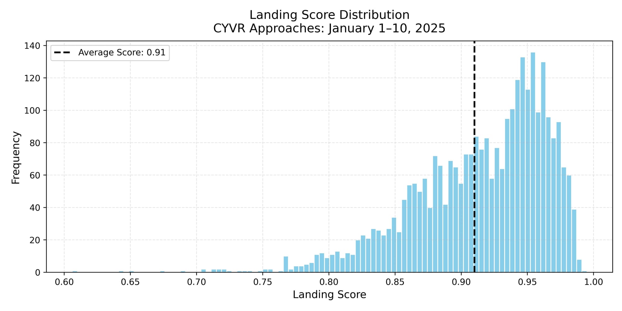
Overall, the results show that most landing scores were quite high, with an average score of 0.91—indicating that virtually all aircraft in our sample closely followed the IFR approach path. While there were a few outliers, the vast majority of flights fell within the 0.80 to 0.95+ range, which is encouraging to see.
2. Altitude Deviations at 6.1 NM from Runway Threshold
As previously noted, 6.1 nautical miles from the runway corresponds to the Final Approach Fix (FAF), where aircraft should be established on a stable descent near 2,000 feet MSL. Reaching this altitude at the FAF is critical, as it ensures proper obstacle clearance and establishes a stable descent path along the standard 3-degree glide slope.
In analyzing the altitude deviations at the FAF across all recorded approaches, we found that the majority of aircraft were slightly above the published altitude—an outcome that aligns with operational best practices. In instrument flying, it is generally preferable for aircraft to be at or slightly above the minimum published altitude rather than below, providing an added margin of safety and supporting a stabilized approach profile.
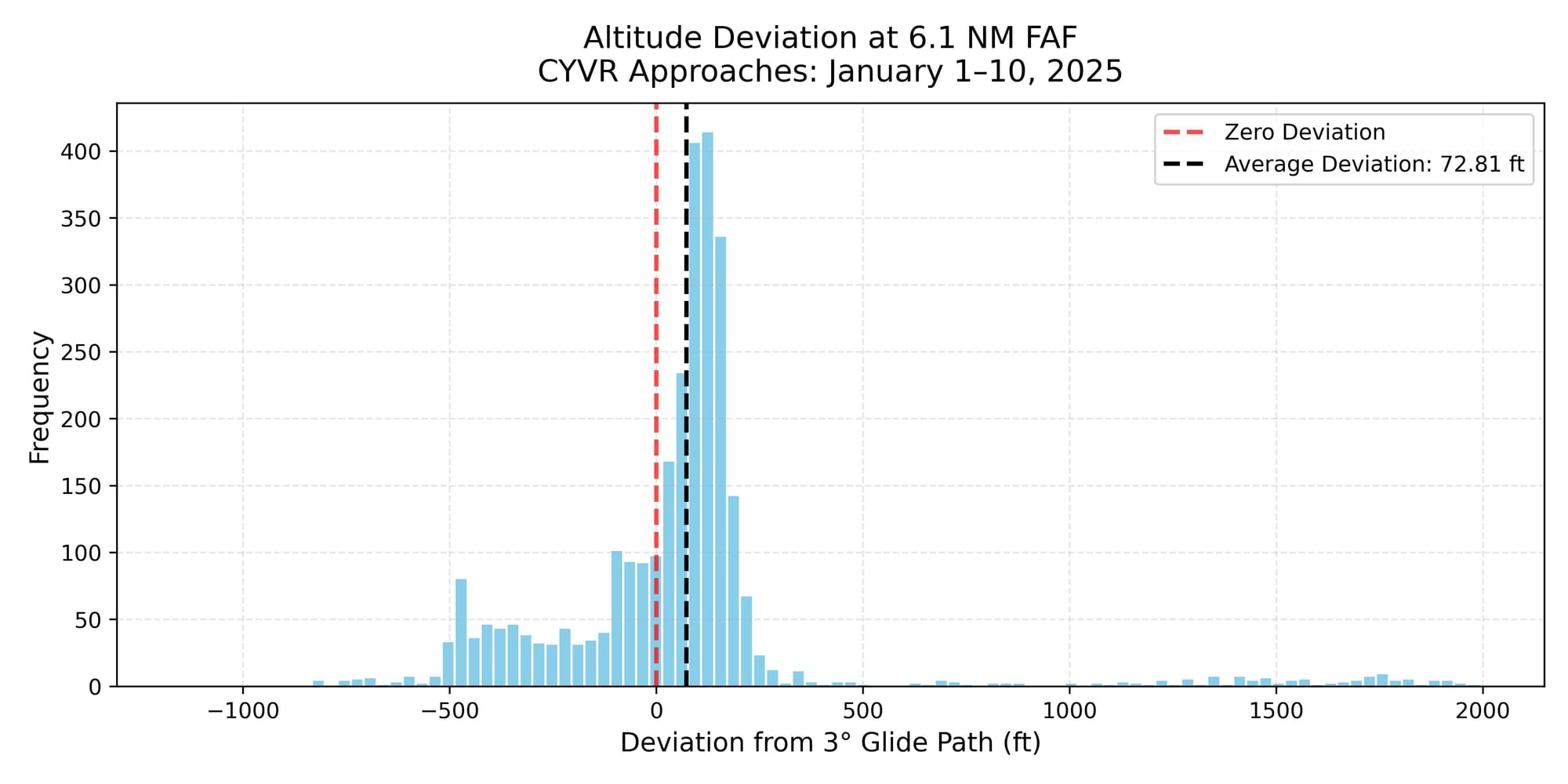
That said, several outliers were observed—flights that were noticeably below the expected FAF altitude, in some cases by several hundred feet. While this falls outside ideal parameters, it’s difficult to attribute these deviations definitively without additional data such as ATC instructions or cockpit-level decision-making. Possible explanations include vectoring at lower-than-published altitudes during sequencing, operational shortcuts during periods of high traffic, or aircraft being cleared for a different type of approach (e.g., visual or RNAV). It’s also possible that some of these deviations are due to noise, data dropouts, or interpolation artifacts in the ADS-B dataset.
In summary, while the overall trend supports stable descent behavior through the FAF, these anomalies highlight the variability present in real-world operations—and the importance of understanding both technical and contextual factors when interpreting glide path conformance.
3. Distribution of Instantaneous Glide Slope at 6.1 NM from Runway Threshold
Another perspective on approach performance is to examine the instantaneous glide slope at 6.1 nautical miles from the runway threshold. In a perfectly stabilized approach, this angle should be close to the theoretical 3 degrees. However, the data reveals that most aircraft tend to fly slightly steeper angles—just above 3 degrees—at this point.
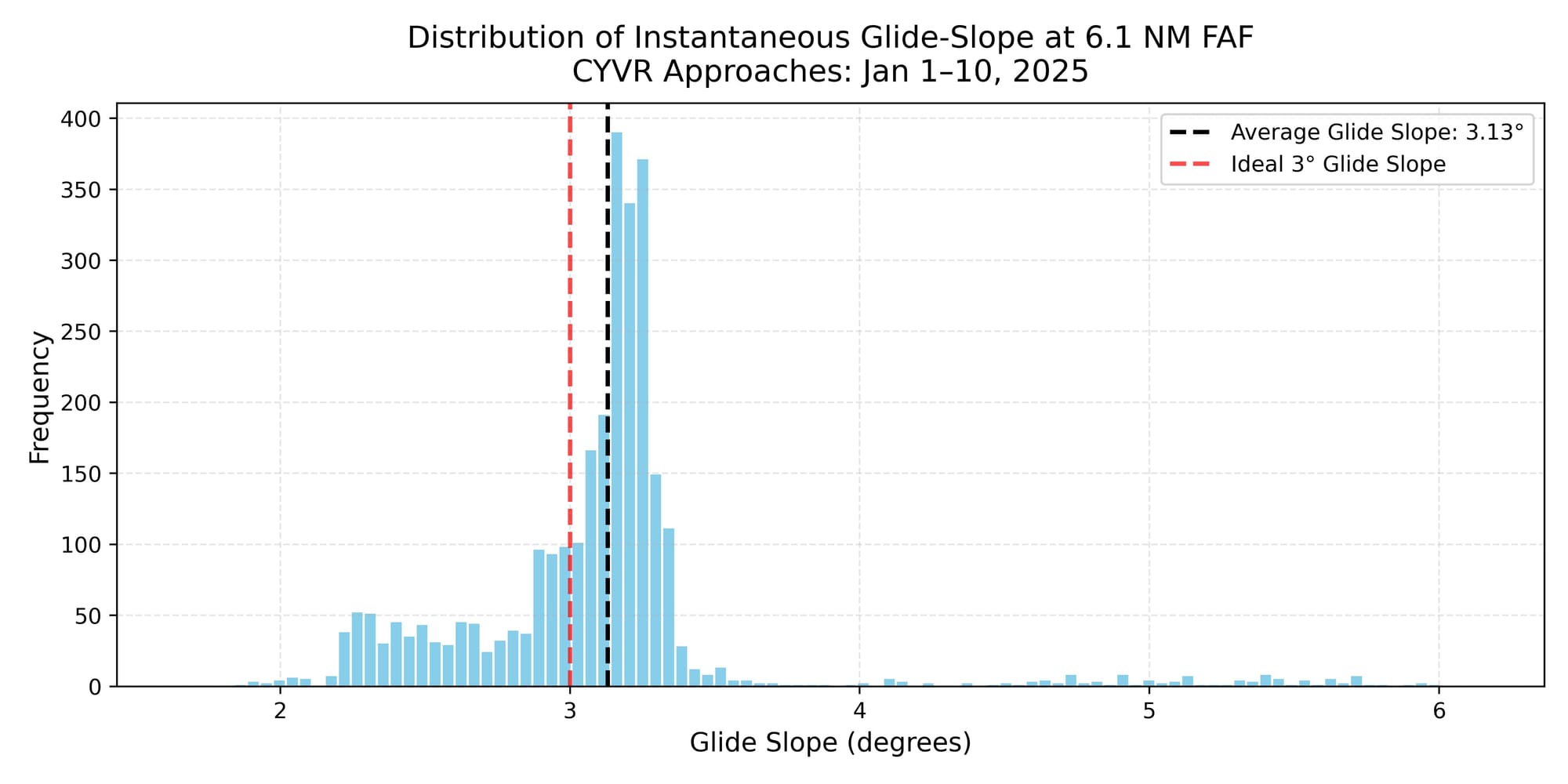
This outcome aligns with earlier observations on FAF altitude deviations. Aircraft arriving slightly above the published FAF altitude would naturally require a slightly steeper descent angle to rejoin and maintain the final approach path.
Overall, the data indicates a high level of consistency in descent profiles, suggesting that pilots are maintaining well-stabilized approaches into CYVR. While the average glide slope is marginally steeper than the theoretical value, this is not a safety concern. Minor variations may result from real-world factors such as ATC vectoring, slight differences in pilot technique, or small inaccuracies in the ADS-B data and glide path calculations.
Taking these factors into account, the overall distribution remains tight and well-centered—reflecting disciplined approach behavior. Notably, while most approaches were stable and uneventful, one particular flight diverged from the pattern and triggered a go-around, offering a valuable case for deeper analysis.
Part 4 | Bonus: Analyzing a Go-Around
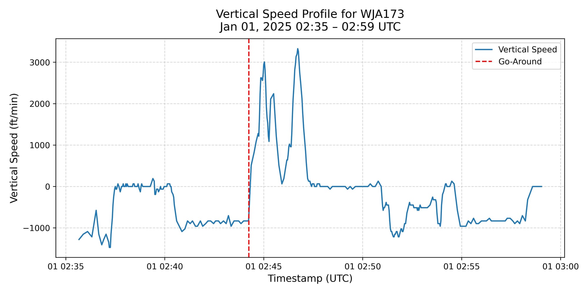
During the analysis, one particular outlier immediately stood out. While reviewing a subset of 100 flights from the morning of January 1st, I noticed an unusual deviation in the flight path of WJA173. The altitude profile strongly suggested a go-around—a situation in which an aircraft on final approach is instructed or chooses to abort the landing and circle back for another attempt. Based on the ADS-B data, the aircraft’s squawk code remained unchanged throughout the maneuver, indicating that the go-around was likely not the result of a serious onboard emergency. Instead, the more plausible cause was a spacing or runway occupancy issue—such as another aircraft still on the runway or delayed in vacating—prompting ATC to instruct the flight crew to execute a missed approach for safety.
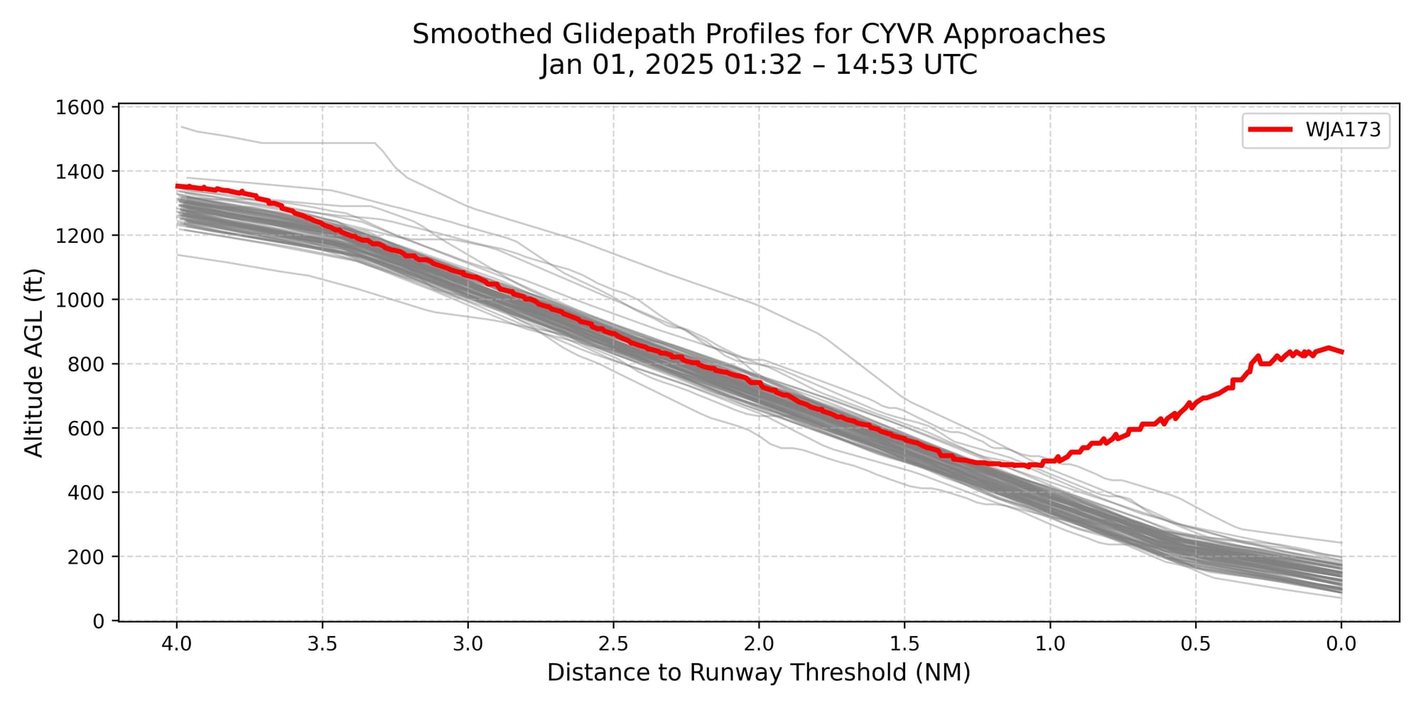
Closer inspection of the altitude and vertical speed data confirms this interpretation. WJA173 was descending steadily on final approach when, at approximately 1,000–1,200 feet AGL, the descent profile abruptly reversed. The aircraft climbed back up to nearly 5,000 feet, with the vertical speed transitioning clearly from a stable descent to a strong positive rate of climb—consistent with a full-power go-around. This was followed by a return to level flight and, later, a controlled descent as the aircraft re-entered the approach phase.
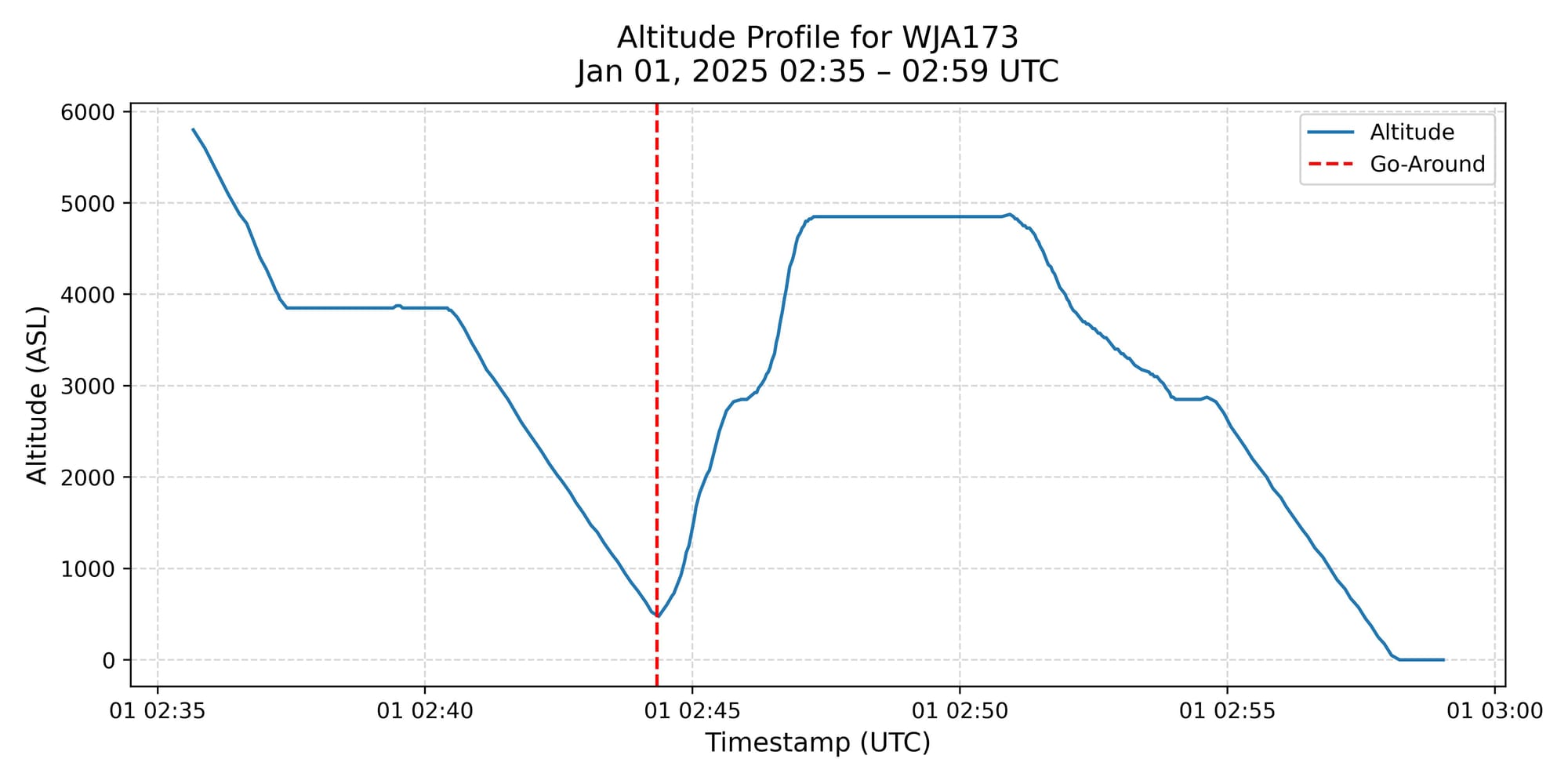
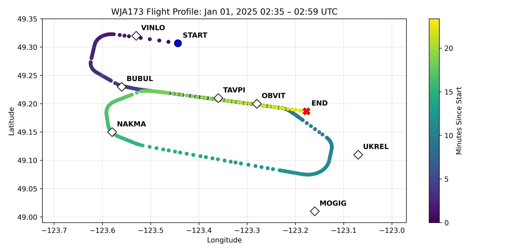
To better understand the sequence, I compared the observed flight path against the published approach procedures. WJA173 was inbound to Runway 08R at CYVR, which supports both ILS and RNAV (GPS) approaches. To clarify the trajectory, I overlaid the RNAV waypoints onto the ADS-B flight path. While the missed approach procedures differ slightly between the ILS and RNAV charts, both call for an initial turn and climb to a designated altitude. In this case, the aircraft’s actual path aligned more closely with the RNAV missed approach, including a segment that passed near NAKMA—a waypoint that does not appear on the ILS chart. This suggests the aircraft was either flying the RNAV procedure or was given direct-to clearances by ATC that bypassed elements of the standard missed approach.
Go-arounds are relatively rare in raw ADS-B datasets, making this case an especially compelling example of real-world dynamics at play. It highlights how unexpected operational scenarios—such as a runway conflict—can unfold in practice, and how data-driven tools can be used not just for performance evaluation, but also to reconstruct and understand rare events that unfold during live operations.
Part 5 | Conclusion
This research highlights how even relatively simple ADS-B datasets—sourced from platforms like FlightRadar24—can yield meaningful insights into real-world flight behavior. By analyzing thousands of approaches into CYVR, we observed that descent profiles are generally stable, pilots maintain safe altitude margins at key points such as the Final Approach Fix, and overall glide slope adherence remains strong, even in the presence of operational complexity. While minor deviations from the ideal 3-degree glide path were common, they can be readily explained by routine factors such as ATC vectoring, traffic sequencing, or small instrumentation and data variances.
These findings also reinforce a broader principle in aviation: while modern cockpits are highly automated, the foundation of safety still rests on pilot skill and judgment. Advanced systems, particularly in precision operations like CAT III ILS landings, significantly reduce workload—but they do not eliminate the need for human oversight. The ability to recognize when something is off—and to act decisively—remains critical.
I experienced this personally during my IFR flight test, when the autopilot failed unexpectedly on final approach. In that moment, no amount of automation could help; being able to hand-fly the ILS accurately and with confidence under pressure made all the difference. Automation is a powerful tool, but it is not a replacement for airmanship. In a world where technology continues to evolve, the mastery of fundamental flying skills remains the last line of defence—and a defining mark of a capable pilot.
Appendix: Haversine Distance Example
To account for the Earth’s curvature when measuring distances between two points, the Haversine formula is commonly used. Rather than calculating simple straight-line (flat-Earth) distances, the Haversine formula provides the shortest path over the globe—also known as the Great Circle distance.
As an illustrative example, consider a transatlantic flight from London Heathrow (LHR) to New York John F. Kennedy (JFK):
- London Heathrow: Latitude 51.47°, Longitude –0.4543°
- New York JFK: Latitude 40.6413°, Longitude –73.7781°
The Haversine formula is:
$d = 2R \arcsin\left( \sqrt{ \sin^2\left( \frac{\Delta\phi}{2} \right) + \cos(\phi_1) \cos(\phi_2) \sin^2\left( \frac{\Delta\lambda}{2} \right) } \right)$
Where:
- $\phi$ = latitude in radians
- $\lambda$ = longitude in radians
- $R = 3440.065$ nautical miles (Earth’s radius)
⚠️ Important: Latitude and longitude must be converted from degrees to radians before using them in the formula.
To calculate the great-circle distance:
- Convert degrees to radians:
- $\phi_1 = 51.47^\circ \times \frac{\pi}{180} \approx 0.898$
- $\phi_2 = 40.6413^\circ \times \frac{\pi}{180} \approx 0.709$
- $\lambda_1 = -0.4543^\circ \times \frac{\pi}{180} \approx -0.00793$
- $\lambda_2 = -73.7781^\circ \times \frac{\pi}{180} \approx -1.2877$
- Compute the differences:
- $\Delta\phi = \phi_2 - \phi_1 \approx -0.189$
- $\Delta\lambda = \lambda_2 - \lambda_1 \approx -1.2798$
- Plug values into the formula and solve.
The computed distance between London Heathrow and New York JFK is approximately 3009 nautical miles.
This example highlights how even relatively “straight” flights must account for the Earth’s curvature over large distances—a principle that the Haversine formula captures cleanly.
While for short final approach segments (e.g., within 10 NM of a runway), this curvature effect is negligible, it becomes essential for longer-range calculations.